NEB using nappy and ase

NEB法は，原子拡散や化学反応など原子の構造的変化の始状態と終状態がわかっていたら，その間の構造を内挿して，イメージを作り，そのイメージ間にバネが働いているとして，全てのイメージをつなげてエネルギー最適化を行うことで，反応のエネルギーバリアを求めるもので，広く使われている．

ASEにはNEB計算を行うモジュールがあるので，PMD_ASE_Calculatorを使ってASEからpmdを呼び出すようにすると，pmd内の力場を使ってNEBを行うことができる．

import nappy
from nappy.interface.ase.pmdrun import PMD_ASE_Calculator as PMDCalc
from ase.mep.neb import NEB
from ase.optimize import FIRE
#...始点構造・終点構造をロード（それぞれ構造最適化は終わっていると仮定）
nsys_ini = nappy.io.read('pmd_ini')
nsys_fin = nappy.io.read('pmd_fin')
ini = nsys_ini.to_ase_atoms()
fin = nsys_fin.to_ase_atoms()
#...内挿してイメージを作成
nimg = 11
images = [ini]
images += [ ini.copy() for i in range(nimg -2)]
images += [fin]
neb = NEB(images)
neb.interpolate(mic=True)
#...全てのイメージにcalculatorを設定
#...（Morse, Coulomb, angularのパラメータファイルが存在していることを仮定）
for image in images:
    image.calc = PMDCalc(force_type=['Morse', 'Coulomb', 'angular'],
                         cutoff_radius=6.0)
opt = FIRE(neb, trajectory='neb.traj')
#...NEB法実行
opt.run(steps=100, fmax=0.05)

こうすうると，次のような出力が出る．

      Step     Time          Energy          fmax
FIRE:    0 18:35:44    -3692.341997        1.067001
FIRE:    1 18:35:44    -3692.971828        0.996428
FIRE:    2 18:35:44    -3694.099314        0.872734
...

各イメージは potential_energy を持っているので，それをプロットする．

xs = []
ergs = []
for i,img in enumerate(images):
    ergs.append(img.get_potential_energy())
    xs.append(i)
ergs = np.array(ergs)
xs = np.array(xs)
 
def spline(x,y,point):  # スプライン曲線で点と点をつなぐ
    from scipy import interpolate
    f = interpolate.Akima1DInterpolator(x, y)
    X = np.linspace(x[0],x[-1],num=point,endpoint=True)
    Y = f(X)
    return X,Y
 
fig, ax = plt.subplots(figsize=(5,5))
xs2, ys2 = spline(xs, ergs, 100)
ax.plot(xs2, ys2-ergs.min(), 'k-', label='Interpolation')
ax.plot(xs, ergs-ergs.min(), 'wo', mec='k', label='Data points')
ax.set_xlabel('NEB image number')
ax.set_ylabel('Energy (eV)')
ax.set_xticks([0,2,4,6,8,10])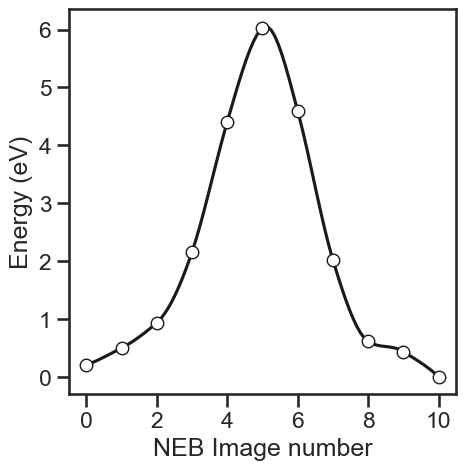

途中構造の確認は，次のようにして途中経過ファイルを出力してOvitoなどで可視化すればよい．

for i,img in enumerate(images):
    nsys = nappy.io.from_ase(img)
    nappy.io.write(nsys, fname=f'dump_{i:02d}')