fp.py or fp --- fit parameters of classical potentials or anything¶

fp.py was migrated to optzer at 2022/12/25. This program will not be updated or maintained any more. Please use optzer instead.

If you are using potential BVSx in in.fitpot, the option is not available in optzer. But the same can be done in optzer. Please see examples/02_pmd_LZP in optzer GitHub repository.

The python program fp.py (or fp) is another program of fitting potential parameters. The fitpot focuses on the neural-network (NN) potential, on the other hand, this fp.py focuses on classical potentials that have much less potential parameters compared to the NN potential, usually less than 100. Since the number of parameters to be optimized is small, fp.py employs meta-heuristic, nature-inspired or Bayesian-optimization method, which can adopt any physical value as a learning target since derivatives of the target values w.r.t. optimizing parameters are not required.

Setup¶

See Install for the setup of nappy. Once nappy is installed, the command fp will be available. fp calls fp.py python program at nap/nappy/fitpot/fp.py, so directory calling fp.py should work as well.

What does fp.py/fp do?¶

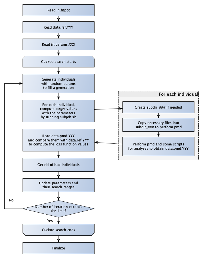
In the fp.py/fp, the following loss function is minimized by optimizing potential parameters,

\[\mathcal{L} = \sum_t \mathcal{L}_t\]

where \(t\) stands for the type of target and it can be anything if it is computed from ab-initio program and MD program using the potential. If the target is the volume of the system,

\[\mathcal{L}_\mathrm{V} = \left( \frac{V_\mathrm{FF} -V_\mathrm{ref}}{V_\mathrm{ref}} \right)^2.\]

If the target is the radial distribution function (RDF),

\[\mathcal{L}_\mathrm{R} = \frac{1}{N_p} \sum_p^{N_p} \left( \frac{\sum_i^{N_\mathrm{R}} (g_{p,\mathrm{FF}}(r_i)- g_{p,\mathrm{ref}}(r_i))^2}{\sum_i^{N_\mathrm{R}} g_{p,\mathrm{ref}}^2(r_i)} \right),\]

where \(N_p\) is the number of RDF pairs to be considered, \(N_\mathrm{R}\) is the number of sampling points of RDF.

To minimize the above loss function, the following methods are available:

Cuckoo search (CS)
Weighted Tree-structured Parzen Estimator (WPE)

The flowchart of fp.py is shown below.

Quick trial with examples¶

There are two examples of fp.py in nap/examples/,

fp_LZP/ -- fitting of parameters of Morse, Coulomb and SW-like angular potentials to RDF, angular distribution function (ADF) and equilibrium volume of Li-Zr-P-O system.
fp_LATP/ -- fitting of parameters of Morse, Coulomb and SW-like angular potentials to RDF, ADF and equilibrium volume of Li-Al-Ti-P-O system.

In either of these two directories, you can try fp.py by running the following command,

$ python /path/to/nap/nappy/fitpot/fp.py --nproc 4 --random-seed 42| tee out.fp

This could take a few minutes using 4 processes. And you can see some output files written by fp.py. See how to discuss result.

You can also do the same as,

$ fp --nproc 4 --random-seed 42 | tee out.fp

Files needed to run fp.py¶

As you can see in nap/examples/fp_LZP/ or nap_examples/fp_LATP/, there are several files needed to run the fp.py program.

in.fitpot -- fp.py configuration file
in.vars.fitpot -- optimizing parameter file
in.params.XXX -- potential parameter files that are not actually used during optimization, except that in.params.Coulomb must exist becuase charge information of each element is read from it.
data.ref.XXX -- Reference data file
subjob.sh -- Shell-script file to perform sub jobs
Files needed to perform sub jobs:
pmdini -- atom configuration file (cell info, positions, and velocities)
in.pmd.NpT -- input file for pmd

Reference data for fp.py¶

Reference data should be stored in files data.ref.XXX where XXX indicates the type of target quantity, such as rdf, adf, vol, etc.

Currently (July 2020), fp.py can run in two different modes,

distribution function (DF)-matching mode -- RDF, ADF, equilibrium volume and lattice constants are adopted as targets.
any-target mode -- any quantity that is computable can be used as a target.

In the DF-matching mode, the reference data formats of these targets are different.

On the other hand, in the any-target mode, the format of reference data is identical in all targets.

Reference data format in DF-matching mode¶

See the format of each target (RDF, ADF, vol and lat) in nap/examples/fp_LZP/.

Reference data format in any-target mode¶

The format of reference data as follows, :

# comment line begins with `#`
#
    100    1.0
    0.1234   0.2345  0.3456  0.4567  0.5678  0.6789
    0.7890   0.8901  0.9012  0.0123  0.1234  0.2345
    ...

Lines begining with # at the head of the file are treated as comment lines.
1st line -- NDAT the number of data, WGT the weight for this target.
2nd line and later -- data, no limitation to the number of entries in a line, but it is recommended to include 6 entries in a line.

Input file in.fitpot¶

Control parameters for fp.py are read from in.fitpot in the working directory. There are some diffierences between DF-matching mode and any-target mode in in.fitpot.

First, in the case of any-target mode, the in.fitpot in the example nap/examples/fp_LATP/ is shown below,

num_iteration      100
print_level         1

fitting_method   cs
sample_directory "./"

match     rdf adf vol
potential   BVSx
# param_files  in.params.Coulomb  in.params.Morse

cs_num_individuals   20
cs_fraction          0.25
update_vrange        10
fval_upper_limit     100.0

specorder  Li Al Ti P O

interactions  7
  Li  O
  Al  O
  Ti  O
  P   O
  Al  O  O
  Ti  O  O
  P   O  O

num_iteration -- Number of iterations (generations) to be computed
print_level -- Frequency of output [default: 1]
fitting_method -- Optimization algorithm [default: cs]
sample_directory -- Directory where the reference data, data.ref.XXX, exist.
match xxx yyy zzz -- List of quantities used as optimization targets
potential -- Potential type whose parameters to be optimized. Currently available potentials are Morse, BVS, and BVSx.
param_files -- Instead of specifying potential, parameter files can be directly specified, which is more flexible and recommended in the version since rev211111.
cs_XXXX -- Parameters related to CS.
cs_num_individuals -- Number of individuals (nests) in a generation.
cs_fraction -- Fraction of abandons in a generation.
update_vrange -- Update variable search range every update_vrange step.
fval_upper_limit -- Upper limit of loss function. The loss functions above this limit is set to this value.
specorder -- Order of species used in reference and MD program.
interaction -- Pairs and triples that are taken into account for optimization.

Parameter file in.vars.fitpot¶

The parameter file in.vars.fitpot contains initial values and ranges of each parameter to be explored.

#  hard-limit:   T
#
  10     6.000   3.000
     1.0000     1.0000     1.0000     1.000    1.000
     0.9858     0.5000     1.5000     0.500    3.000
     0.8000     0.5000     1.5000     0.500    3.000
     0.9160     0.5000     1.5000     0.500    3.000
     1.1822     0.5000     5.0000     0.100   10.000
     2.1302     1.5000     3.0000     0.100   10.000
     1.9400     1.5000     2.5000     0.100   10.000
     4.1963     3.0000     8.0000     0.100   10.000
     2.5823     1.5000     3.0000     0.100   10.000
     1.4407     1.2000     2.0000     0.100   10.000

Lines begin with # at the head of the file are treated as comment lines.
hard-limit: T in comment line is a optional setting. The hard-limit set additional hard limit for parameters for automatic update of the search range.
1st line -- Number of optimizing parameters NVAR, cutoff radius for 2-body potential RCUT2, and cutoff for 3-body potential RCUT3, respectively.
2nd line and later -- initiall value, soft-limit (lower and upper), hard-limit (lower and upper), respectively. If hard-limit: F (hard-limit is not set), entries for hard-limit are not required in a line.

Parameter files in.params.XXX used to run subjobs¶

This is only the case when specifying param_files instead of specifying potential in in.fitpot.

The key-words, {p[#]} where # is a number, in the parameter files specified by param_files are to be replaced with the optimizing parameters in in.vars.fitpot. The example of in.params.Morse is as follows:

# cspi, cspj,    D,      alpha,     rmin
  Li    O     {p[4]}     {p[5]}     {p[6]}
  Zr    O     {p[7]}     {p[8]}     {p[9]}
  P     O     {p[10]}    {p[11]}    {p[12]}

Therefore, using param_files, users can optimize parameters of not only pmd but also of any program with fp.py.

Subjob script subjob.sh¶

The subjob.sh is used to perform MD runs and extract data for evaluating the loss function of each nest (individual). :

#!/bin/bash
#=======================================================================
#  Script to be called from fp.py to perfom pmd simulation
#  and to extract RDF, ADF, and volume data.
#
#  Usage:
#    $ run_pmds.sh
#=======================================================================

#...copy filed required for pmd calculation
cp ../in.pmd* ../pmdini ./

#...cd to the directory and clean up
rm -f dump_* out.* data.pmd.*

#...NpT MD
cp in.pmd.NpT in.pmd
pmd 2>&1 > out.pmd.NpT
head -n166 out.pmd.NpT
tail -n20 out.pmd.NpT
echo "NpT-MD done at" `date`
#...extract rdf, adf, vol and rename files
python ~/src/nap/nappy/rdf.py -d 0.05 -r 5.0 --gsmear=2 --skip=80 --specorder=La,Li,F --pairs=La-F,Li-F --out4fp -o data.pmd.rdf dump_* 2>&1
python ~/src/nap/nappy/adf.py --gsmear=2 --triplets=Li-F-F --out4fp --skip=80 -o data.pmd.adf dump_* 2>&1
python ~/src/nap/nappy/vol_lat.py --out4fp --skip=80 dump_* 2>&1
echo "post-processing done at" `date`

--pairs and --triplets should be correctly set in rdf.py and adf.py as well as --specorder options.
--out4fp option is required to write any-target mode format of reference data. On the other hand, in the case of DF-matching mode, --out4fp option should not be used.

in.pmd file in the subjob¶

Here is an example of in.pmd file used in subjob of each individual (nest), acually named in.pmd.NpT in nap/examples/fp_LATP.

max_num_neighbors         200

time_interval              2.0
num_iteration            10000
min_iteration               5
num_out_energy           1000

flag_out_pmd                1
num_out_pmd               100
flag_sort                   1

force_type           Morse Coulomb angular
cutoff_radius                6.0
cutoff_buffer                0.3

flag_damping                 0
damping_coeff                0.99
converge_eps                 1.0e-05
converge_num                 3

initial_temperature        300.0
temperature_control        Langevin
temperature_target         1  300.0
temperature_relax_time     50.0
remove_translation         1

factor_direction          3 1
    1.00   1.00   1.00

stress_control              vc-Berendsen
pressure_target              0.0
stress_relax_time           50.0

See Input file: in.pmd for detailed meaning of the input file.

In short, this in.pmd.NpT is going to perform a MD simulation of 10,000 steps with Morse, Coulomb and angular potentials at 300 K under NpT condition.

And from the output pmd_### files, target quantities are extracted using some python scripts as described in subjob.sh. Those python scripts create data.pmd.XXX files as output and fp.py is going to read those data files to evaluate the loss function of each individual (nest).

Run fp.py¶

$ python ~/src/nap/fitpot/fp.py --nproc 4 | tee out.fp

--nproc sets number of processes used for the evaluation of individuals.
--subjob-script option sets which script file is used for to perform subjob. [default: subjob.sh]
--subdir option sets the prefix of directories where the subjobs are performed. [default: subdir]

Results and outputs¶

Files and directories created by fp.py are,

out.fp -- Standard output.
out.cs.generations -- Information of generations.
out.cs.individuals -- Information of all the individuals.
in.vars.fitpot.#### -- Parameter file that is written whenever the best individual is updated.
in.vars.fitpot.best -- Parameter file of the best individual in the run.
subdir_### -- Directories used for the calculations of individuals. You can remove these directories after the run.

Convert fp.py parameter file to pmd parameter files¶

$ python ~/src/nap/nappy/fitpot/fp2prms.py BVSx in.vars.fitpot.best

This command will create in.params.Morse, in.params.Coulomb and in.params.angular files (the keyword BVSx means that these 3 potentials).

Visualize the evolution of optimization¶

One can plot loss function values of all the individuals appeared during optimization as a function of generation using gnuplot as, :

$ gnuplot
gnuplot> set ylabel 'Loss function value'
gnuplot> set xlabel 'Generation'
gnuplot> p 'out.cs.generations' us 1:3 w p pt 5

Check if the loss function converges.
Check that the minimum loss function value is sufficiently small (below 0.01 per target would be good enough).

Visualize the distribution of each parameters¶

You can plot the parameter values of all the individuals using the data in out.cs.individuals as,

$ gnuplot
gnuplot> p 'out.cs.individuals' us 7:2 w p t 'D (Li-S)', '' us 8:2 w p t 'alpha (Li-S)', '' us 9:2 w p t 'Rmin (Li-S)'